25 Agents Walk Into a Market: How to Build AI-Powered Trading Infrastructure

I’ve had a pile of quantitative finance posts sitting in my Instagram saved tab for months — stochastic calculus breakdowns, agent architecture diagrams, volatility modeling walkthroughs. Individually they’re great content. But when I ran them all through DejaViewed and the AI started cross-linking everything, something clicked. These posts aren’t about individual models. They’re pieces of something bigger — a multi-agent debate system where 25+ specialized AI agents argue with each other before any trade goes through.

I got pretty deep into this rabbit hole. Here’s the whole thing — the individual quant models, how they’re organized into 4 layers, and how the debate framework ties them together. All of it comes from real people sharing real implementations on Instagram, not textbooks.

The Architecture: 25 Agents, 4 Layers, Real-Time Debate

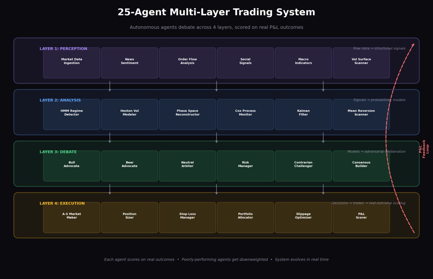
This started with a post from @marc.kaz about a system where 25+ autonomous agents debate every trading day across 4 layers and evolve in real time. Each agent runs a different market model. They don’t just vote — they argue, present evidence, and get scored on real P&L. Agents that keep getting it wrong lose influence. Agents that find edge get louder.

View the original post →

What grabbed me is that this isn’t ensemble modeling with static weights. The agents’ authority shifts based on market conditions. The four layers each handle something different:

• Layer 1 — Regime Detection: What market are we in? (HMMs, trend classifiers)
• Layer 2 — Pricing & Volatility: What’s the fair price and risk surface? (Heston, Black-Scholes extensions)
• Layer 3 — Hidden Dynamics: What’s the underlying dynamical regime? (Phase space reconstruction, Lyapunov analysis)
• Layer 4 — Execution: How do we enter/exit optimally? (Avellaneda-Stoikov, Cox process monitoring)

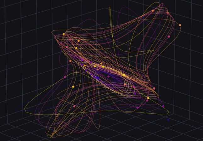
During a quiet bull market, Layer 1’s trend-followers dominate. When a regime shift hits, the HMM agents gain authority because they caught it first. Layer 2’s Heston agent simultaneously flags vol surface changes. Layer 3’s PSR agent sees it as a chaotic transition — like the attractor in the hero image above breaking from its orbit. And Layer 4 widens execution spreads to protect capital. All of this happens autonomously.

Layer 1: Regime Detection — Hidden Markov Models

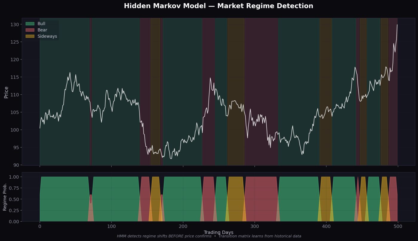
Before you can trade anything, you need to know which market you’re in. Hidden Markov Models treat the true market regime (bull, bear, recovery, crisis) as a hidden state that produces the data we can actually measure — returns, volume, volatility.

@quant.traderr has a great breakdown of this. HMMs use the Baum-Welch algorithm to learn transition probabilities and the Viterbi algorithm to decode the most likely state sequence. The part that got me: it identifies low-vol bull, high-vol bear, and recovery regimes automatically — way better than moving average crossovers or anything else that lags.

How HMMs Work in Trading

1. Define observable features: daily returns, realized volatility, volume ratio
2. Choose number of hidden states: typically 3-5 (bull, bear, recovery, crisis, transition)
3. Train with Baum-Welch: learns emission probabilities (what each state “looks like”) and transition matrix (how likely state changes are)
4. Decode with Viterbi: given today’s observables, what’s the most likely current regime?
5. Condition strategy: different agents activate depending on detected regime

from hmmlearn.hmm import GaussianHMM
import numpy as np

# Features: [returns, volatility, volume_ratio]
features = np.column_stack([returns, volatility, volume_ratio])

model = GaussianHMM(n_components=3, covariance_type="full", n_iter=100)
model.fit(features)

# Decode current regime
hidden_states = model.predict(features)
current_regime = hidden_states[-1]  # 0=bull, 1=bear, 2=recovery

In the multi-agent system, the HMM agent broadcasts its regime call to every other agent. A shift from bull to bear triggers a cascade across all four layers: Layer 2’s Heston agent recalibrates for higher vol-of-vol, Layer 3’s PSR agent starts watching for chaotic transitions, and Layer 4’s market maker widens spreads immediately.

Layer 2: Volatility Surface — The Heston Model

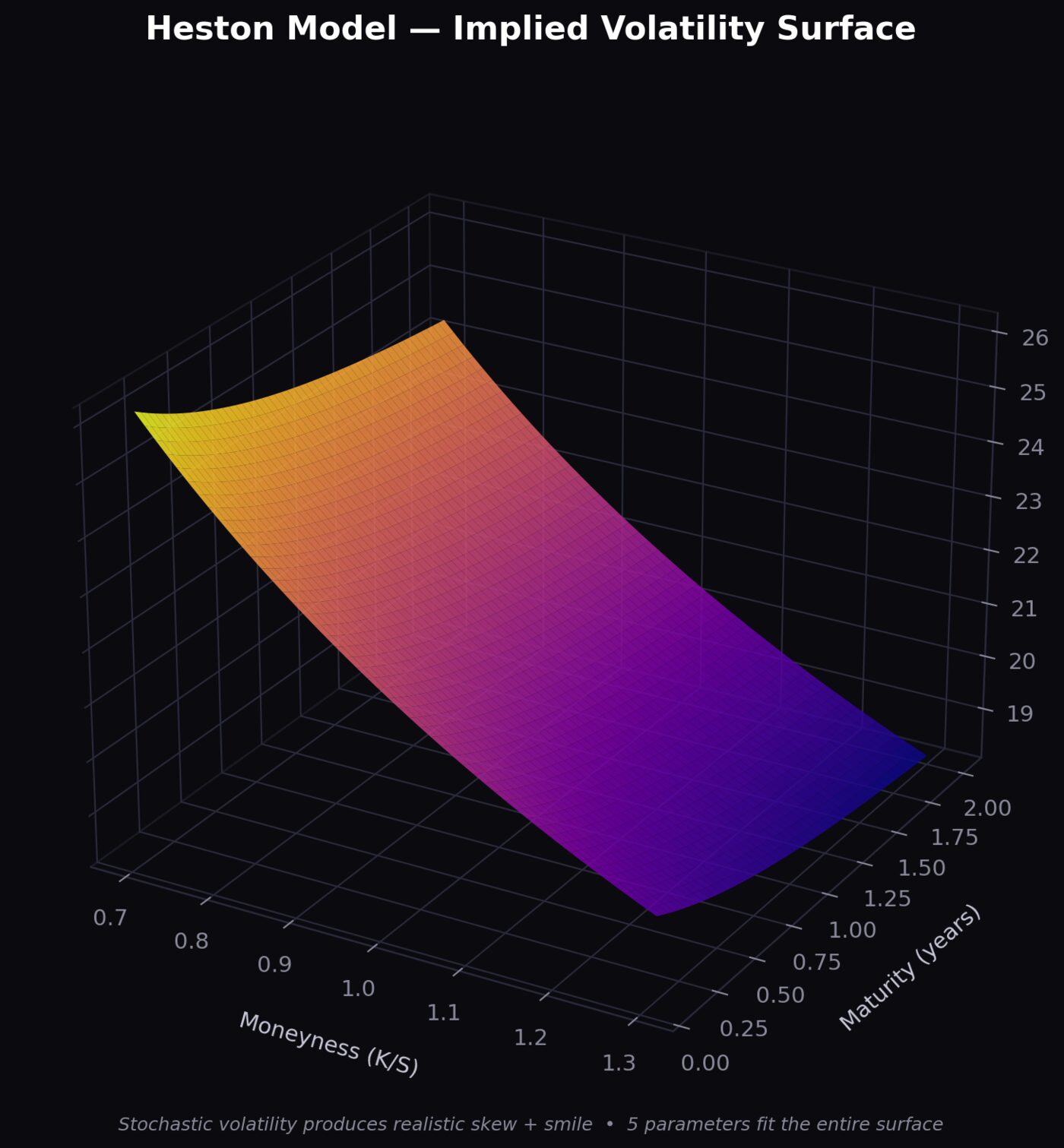
Black-Scholes assumes volatility is constant. Anyone who’s traded options knows that’s wrong — the volatility smile and skew exist precisely because volatility is stochastic. The Heston Model fixes this by modeling volatility itself as a mean-reverting process, and it gives you a closed-form solution that actually matches what you see in the market.

Heston’s Five Parameters

• v₀ — initial variance (current vol level)
• θ — long-run variance (where vol mean-reverts to)
• κ — speed of mean reversion (how fast vol returns to θ)
• σ — vol of vol (how volatile is volatility itself)
• ρ — correlation between asset returns and vol (typically negative — the “leverage effect”)

The Heston agent continuously calibrates these 5 parameters against live options data. When the vol surface changes shape — steeper skew, flatter smile — it’s signaling something that complements Layer 1’s HMM. These two agents disagree a lot, and that’s the whole point. A vol surface screaming “danger” while the HMM still says “bull” is exactly the kind of early warning the debate system exists to catch.

# Heston characteristic function for option pricing
def heston_char_func(u, S, K, T, r, v0, theta, kappa, sigma, rho):
    d = np.sqrt((rho*sigma*u*1j - kappa)**2 + sigma**2*(u*1j + u**2))
    g = (kappa - rho*sigma*u*1j - d) / (kappa - rho*sigma*u*1j + d)

    C = r*u*1j*T + (kappa*theta/sigma**2) * \
        ((kappa - rho*sigma*u*1j - d)*T - 2*np.log((1-g*np.exp(-d*T))/(1-g)))
    D = ((kappa - rho*sigma*u*1j - d)/sigma**2) * \
        ((1-np.exp(-d*T))/(1-g*np.exp(-d*T)))

    return np.exp(C + D*v0 + 1j*u*np.log(S))

Layer 3: Hidden Dynamics — Phase Space Reconstruction

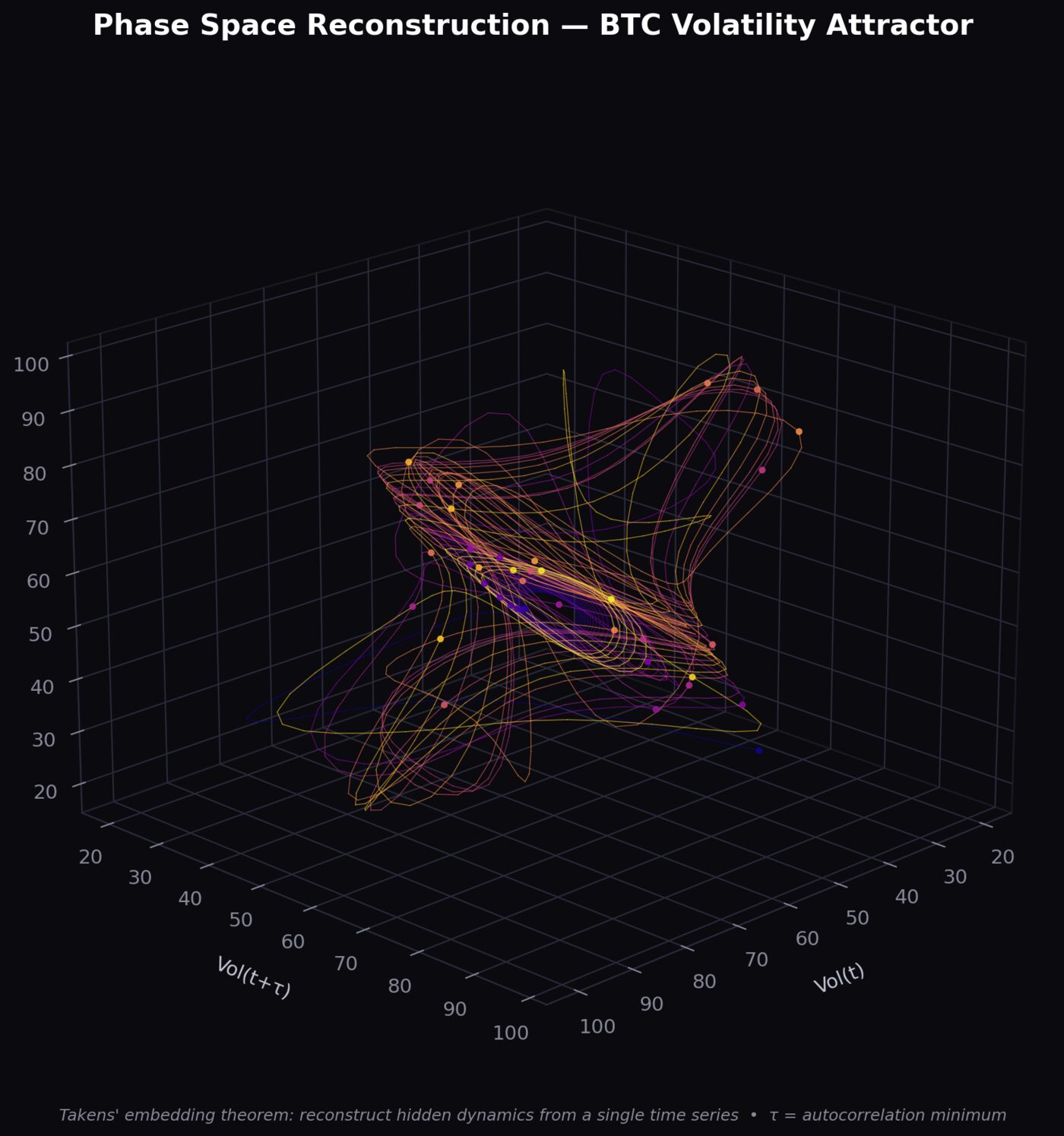
This is where it gets interesting. Phase Space Reconstruction comes from chaos theory — specifically Takens’ embedding theorem, which proves you can reconstruct a full dynamical system from a single time series if you pick the right embedding dimension and time delay.

That swirling attractor at the top of this post? That’s what market dynamics actually look like when you unfold a flat price chart into its true multi-dimensional phase space. The orbits, the dense regions, the chaotic escapes — that’s not noise. It’s structure. I stared at this one for a while.

Applied to BTC volatility with time delay τ=3, PSR unfolds the 1D price series into a manifold that shows whether the market is sitting in a stable attractor (predictable) or going through a chaotic transition (regime shift in progress). This gives Layer 3 a completely different perspective than Layer 1’s HMM. The HMM tells you “we’re in a bear market.” PSR tells you “the system is approaching a bifurcation point” — a regime shift is about to happen, not that it already has. That distinction matters.

# Phase Space Reconstruction via time delay embedding
def embed_time_series(x, tau=3, dim=3):
    """Takens' embedding: reconstruct phase space from scalar time series.

    Args:
        x: 1D time series (e.g., realized volatility)
        tau: time delay (use mutual information to optimize)
        dim: embedding dimension (use false nearest neighbors)
    """
    n = len(x) - (dim - 1) * tau
    embedded = np.zeros((n, dim))
    for i in range(dim):
        embedded[:, i] = x[i*tau : i*tau + n]
    return embedded

# Reconstruct BTC volatility phase space
phase_space = embed_time_series(btc_volatility, tau=3, dim=3)

# Compute largest Lyapunov exponent — positive = chaos
from nolds import lyap_r
lyap = lyap_r(btc_volatility)
print(f"Lyapunov exponent: {lyap:.4f}")  # > 0 means chaotic

Layer 4: Execution — Avellaneda-Stoikov Market Making

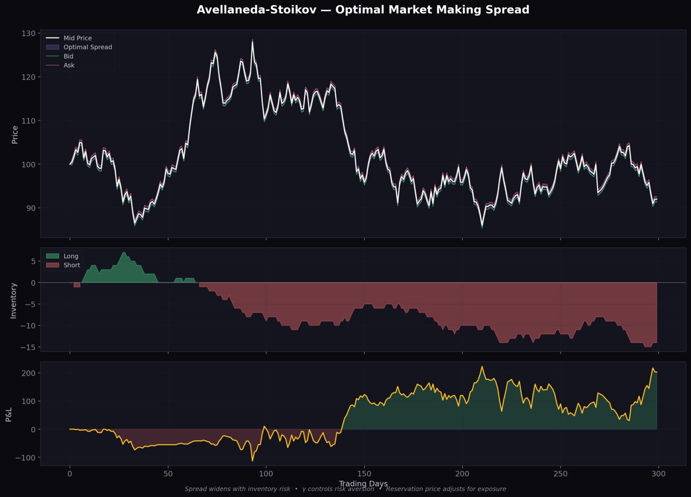
Once Layers 1-3 have their picture — what regime we’re in, what the vol surface looks like, whether the dynamics are stable or chaotic — the Avellaneda-Stoikov agent in Layer 4 handles the actual trading. It solves the market making problem: what bid-ask spread should you quote given your inventory, the asset’s volatility, and how much time you have left?

The Core Formula

The reservation price (where you’d ideally trade) shifts from the mid-price based on inventory risk:

# Avellaneda-Stoikov reservation price and optimal spread
def optimal_spread(mid_price, inventory, volatility, gamma, T_remaining):
    """
    gamma: risk aversion parameter
    T_remaining: time until end of trading session
    """
    # Reservation price: adjusted mid based on inventory
    reservation = mid_price - inventory * gamma * volatility**2 * T_remaining

    # Optimal spread: wider when vol is high, time is short
    spread = gamma * volatility**2 * T_remaining + (2/gamma) * np.log(1 + gamma/kappa)

    optimal_bid = reservation - spread/2
    optimal_ask = reservation + spread/2

    return optimal_bid, optimal_ask, reservation

The A-S agent takes signals from every upstream layer. Layer 1’s HMM says “bear regime” → widen spreads. Layer 2’s Heston agent sees rising vol-of-vol → bump the risk aversion parameter. Layer 3’s PSR agent flags a chaotic transition → cut position sizes. Every parameter in the execution formula is conditioned on what the layers above are seeing.

The Cross-Layer Glue: Cox Process for Event Clustering

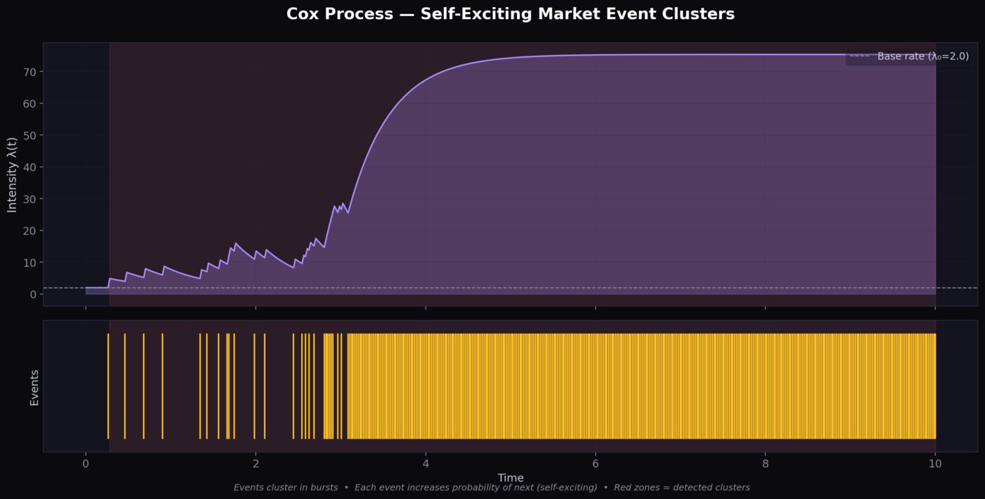
Regular Poisson processes assume events arrive at a constant rate. Markets don’t do that — trades cluster, vol spikes cascade, order flow comes in waves. The Cox Process uses a random intensity to model this burstiness, and it operates as cross-layer infrastructure — monitoring event intensity and alerting agents in all four layers at once.

When intensity spikes, every layer responds: Layer 1’s HMM increases update frequency, Layer 2’s Heston widens confidence intervals, Layer 3’s PSR watches for attractor destabilization, Layer 4’s market maker widens spreads. The self-exciting variant (Hawkes process) adds a feedback loop where each event increases the chance of more events — which is basically how flash crashes and momentum ignition actually work.

Putting It All Together

So that’s each layer. Here’s how data actually flows through them. The architecture diagram earlier shows what the layers are; this one shows how they connect:

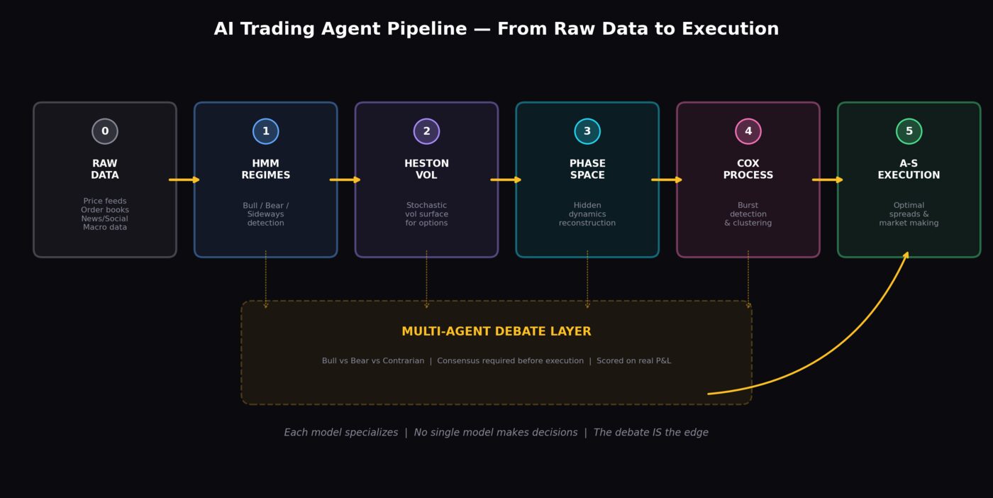
1. Data Ingestion: Market data (price, volume, order book, options chain) streams in
2. Layer 1 — Regime Detection: HMM agents decode current market state
3. Layer 2 — Pricing: Heston agents calibrate the vol surface
4. Layer 3 — Dynamics: PSR agents reconstruct phase space and check for chaos
5. Cross-Layer: Cox Process monitors event intensity and alerts all layers during bursts
6. Debate Layer: Agents present assessments with confidence scores. Disagreements get surfaced. A meta-agent aggregates weighted votes based on track records
7. Decision: Aggregated signal determines position direction, size, and timing
8. Layer 4 — Execution: A-S market maker handles entry/exit, conditioned on everything upstream
9. Scoring: Real P&L gets attributed back to each agent, updating their influence weights

That phase space attractor at the top — that’s what Layer 3 agents are watching constantly. When those orbits are tight and stable, the system is predictable. When they spiral outward, Layer 3 screams “regime shift incoming” and the whole debate system recalibrates. No single model has to be right. The system just needs the right agent to be loud at the right moment. That’s what makes this architecture so compelling — it mirrors how you’d want a team of analysts to work, except they never sleep and they score each other on actual outcomes.

Implementation Roadmap

If you want to build this, here’s how I’d sequence it:

Phase 1: Build Layer 1 — Regime Detection (Week 1-2)

• Implement HMM regime detection on historical data
• Validate against known regime shifts (COVID crash, 2022 bear, 2024 bull)
• Build the data pipeline and backtesting framework

Phase 2: Build Layers 2 & 3 — Pricing + Dynamics (Week 3-4)

• Calibrate Heston model on live options data (Layer 2)
• Implement PSR with optimized τ and embedding dimension (Layer 3)
• Add Cox process monitoring for event intensity (cross-layer)

Phase 3: Build the Debate Framework (Week 5-6)

• Build the agent communication protocol connecting all layers
• Implement weighted voting with track-record scoring
• Add disagreement detection and escalation logic

Phase 4: Build Layer 4 — Execution (Week 7-8)

• Implement A-S market maker with regime-conditioned parameters from Layers 1-3
• Paper trade the full 4-layer system
• Build monitoring dashboard and per-agent P&L attribution

Prerequisites

This is a hard build. You’ll need:

• Python — NumPy, SciPy, hmmlearn, nolds (for Lyapunov exponents)
• Basic stochastic calculus — Itô’s lemma, Brownian motion, CIR process
• Market data API access — real-time and historical (Polygon.io, Alpaca, or similar)
• Options data — for Heston calibration (CBOE, Deribit for crypto)
• Familiarity with at least one quant model before trying the full system

Creators to Follow

All of this came from two people who are consistently putting out great stuff:

• @marc.kaz — the multi-agent architecture and debate system design
• @quant.traderr — all five quant models (HMM, Heston, PSR, A-S, Cox). Every post is S or A tier. Easily one of the best quant educators on Instagram.

---

This post was built from the AI Trading Agents deep dive on DejaViewed — my curated catalog of 437 saved Instagram posts across 14 collections, cross-linked and analyzed by AI. Read more about how DejaViewed works, browse the full catalog, explore the knowledge graph, or check out the other deep dive guides.

---

Update: What I Found When I Actually Tried to Build This

Published: May 6, 2026

After writing the post above, I spent a full evening doing what I should have done first — pulling papers, reading repos, cross-referencing every claim, and comparing everything against my own live trading system that runs 26 bots across 5 divisions on Hyperliquid. Here’s what’s real, what’s not, and what I actually built instead.

The Big Realization: Two Incompatible Paradigms

The original post stitches together content from two creators describing fundamentally different things.

@quant.traderr presents classical quantitative models — HMMs, Heston stochastic volatility, Phase Space Reconstruction, Avellaneda-Stoikov market making. Deterministic math on numerical time series. Numerical signals out.

@marc.kaz (ATLAS-GIC) presents an LLM-based agent debate system — 25+ Claude Sonnet prompts generating text recommendations, scoring them against outcomes, evolving through Darwinian selection.

These are not the same thing. You can’t plug an HMM output into an LLM debate and call it “Layer 1 feeds Layer 4.” They’re architecturally incompatible as described. The honest framing: two valid approaches to beating the market, solving it in completely different ways.

Layer-by-Layer Reality Check

Layer 1: Hidden Markov Models — Real But Redundant

The theory is sound. Hamilton (1989) established Markov-switching models for regime detection. The math works. hmmlearn is production-quality.

The problems nobody mentions on Instagram:

• Detection lag. HMMs detect regime shifts AFTER they happen. By the time you’re confident it’s a bear market, the crash already happened.
• State count is arbitrary. No principled way to choose 2, 3, or 4 states. BIC and AIC often disagree.
• Simpler methods work just as well. A 20-day rolling volatility estimate captures most of what a 3-state Gaussian HMM captures. My own system uses a Kaufman Efficiency Ratio + multi-timeframe direction gate — and we explicitly tested HMM-adjacent approaches and found them “redundant with rv_z or impractical.”
• Transaction costs eat regime alpha. Regimes last months to years. 2-6 trades per year. The edge per trade must be enormous to overcome whipsaw.

Verdict: Educational content ✓. Revolutionary trading edge ✗.

Layer 2: Heston Stochastic Volatility — Wrong Market

Heston (1993) is a genuine masterpiece — closed-form solution for option pricing with stochastic volatility. But here’s the thing: it’s for option pricing. It models the implied volatility surface. It requires options chain data.

If you’re trading crypto perpetual futures (like I am on Hyperliquid), there’s no options surface to calibrate, no implied volatility to extract, no vol smile to model. I found zero published evidence that Heston parameter time series generate alpha in directional spot/perp trading.

Verdict: Brilliant math, wrong application. Only relevant if you’re trading options on Deribit.

Layer 3: Phase Space Reconstruction — I Already Do This (Better)

This was the most interesting discovery. The article presents Takens’ embedding theorem as a way to detect regime shifts before they happen. My system already implements persistent homology on phase-space trajectories, recurrence quantification analysis, information geometry, Koopman operator analysis, and Hurst exponent analysis. The article’s “Layer 3” is the introductory textbook version of what I’m already running with four different mathematical lenses.

What the literature actually says: Moving Lyapunov exponents DO spike before major crashes (Tsakonas et al., 2022). TDA-based filters can reduce drawdowns by ~50% (Levine, 2026, SSRN). But for directional alpha? Zero papers with verified live trading P&L.

The honest conclusion from Hsieh (1991): ARCH effects explain observed nonlinearity. Not deterministic chaos. Markets are high-dimensional stochastic systems with occasional phase transitions. The tools detect the transitions — they don’t predict the direction.

Verdict: Real. I use it. But it’s a risk filter, not an alpha generator.

Layer 4: Avellaneda-Stoikov — Wrong Paradigm Entirely

A-S solves a beautiful problem: what spread should a market maker quote? But my system is directional — taking positions, earning from price movement. These are opposite paradigms. You can’t bolt A-S onto a directional system without a complete architectural redesign, and you’d be competing against Wintermute and Jump with sub-millisecond latency.

If you want market making on Hyperliquid, Hummingbot has a production A-S implementation. But it’s a completely different business.

Verdict: Legitimate math, wrong application for directional trading.

The Industry Reality

I searched exhaustively for deployed multi-agent LLM trading systems with verified live returns:

System	Live Money?	Reality
TradingAgents (UCLA/MIT)	No	“Not intended as financial advice”
ai-hedge-fund (43K stars)	No	“Does not actually make trades”
HedgeAgents (claims 70% annual)	No	Backtest only
ATLAS-GIC	Claims yes	Unaudited self-report
AutoGPT/CrewAI trading bots	No	All educational/experimental

Zero verified multi-agent LLM trading systems with audited live P&L exist in the public domain as of May 2026.

The one legitimate “multi-agent” system that works? Numerai — thousands of data scientists submitting predictions ensembled with stake-weighted averaging. $100M+ AUM. But they don’t use LLMs — they use traditional ML models.

The Real Gold: ATLAS Operational Patterns

While the quant layers were mostly inapplicable, ATLAS’s operational architecture turned out to be genuinely interesting. Not the LLM debate gimmick — the meta-learning patterns:

1. Darwinian Weight System. Each agent has a weight (0.3–2.5). Top quartile gets ×1.05 daily. Bottom gets ×0.95. Good agents get louder. Bad ones get quieter. My application: dynamically weight my 5 trading divisions by rolling Sharpe instead of equal-weighting.
2. Autoresearch Loop. Identify worst agent → one targeted modification → 5 days to prove itself → keep or revert. Over 378 days: 54 modifications, 16 kept (30% survival). My application: monthly parameter tuning on my worst bot. One change, 30 days, keep or revert.
3. Emergent Regime Detection. Multiple agent cohorts trained on different regimes. The weight differential between cohorts IS the regime signal. They didn’t build a detector — it emerged. My application: my divisions ARE cohorts. Which division outperforms IS the regime signal. Zero additional complexity.
4. The CIO Bottleneck. ATLAS independently downweighted its own portfolio manager to minimum weight. Signal generation wasn’t the problem — synthesis was. My lesson: stop adding signals. Fix the orchestration layer.

What I Actually Built Instead

Rather than building a 25-agent debate system, I asked: what would actually help my live trading system right now?

The answer was a shadow signal tracker — a system that logs every trade signal that gets BLOCKED by my position limits, then tracks what those trades WOULD have earned. This answers the real question: are my constraints helping or hurting me?

Within hours of deploying: 7 signals blocked by my MTF direction gate (shorts blocked because macro trend was bullish). The phantom positions are now tracking. In a few weeks, I’ll know whether my limits are protective or restrictive.

That’s the difference between theory and practice. Theory says “build 25 agents.” Practice says “measure whether your existing constraints are correct.”

Key Takeaways

1. Multi-agent debate is 80% marketing, 20% real. The 20%: ensemble methods reduce variance. Calling it “debate” vs “weighted average” is branding.
2. Most quant models in the original post solve problems I don’t have. Heston needs options. A-S needs market making. HMM is redundant with simpler methods.
3. Phase Space Reconstruction is real and I use it — but it’s a risk filter, not an alpha generator.
4. The operational patterns from ATLAS are genuine gold: Darwinian weighting, autoresearch loops, emergent regime detection.
5. No one has proven LLM agents trade better than rules-based systems in live markets. Rules win on speed, cost, determinism, and auditability.
6. The gap between “fascinating theory” and “makes money in production” is enormous. Papers optimize forecasting accuracy. Production systems optimize risk-adjusted returns after costs.
7. Measure before you build. My shadow tracker will reveal more in 2 weeks than any theoretical architecture ever could.

The Creators — Verified Credentials

In the interest of intellectual honesty: @quant.traderr has no verifiable academic credentials, papers, or institutional affiliation. “Turning 9-to-5ers into Algo-Traders.” Educational content creator — the math is correct, but treat as education, not authority. @marc.kaz has no published academic work. The ATLAS repo is real and substantial (1,700+ stars), but no audited track record. This doesn’t mean they’re wrong — it means verify everything independently. Which I did.

Papers & Repos Referenced

Foundational: Hamilton (1989) — regime switching. Heston (1993) — stochastic vol. Takens (1981) — embedding theorem. Avellaneda & Stoikov (2008) — market making. Bacry et al. (2015) — Hawkes processes in finance.

Key negative results: Hsieh (1991) — ARCH explains nonlinearity, not chaos. Tsakonas et al. (2022) — Lyapunov spikes precede crashes but don’t predict direction. Guttal et al. (2016) — critical slowing down fails for recent crashes.

Repos: ATLAS-GIC (1.7K stars) · karpathy/autoresearch (79K stars) · MiroFish (59K stars) · Hummingbot (~15K stars) · hmmlearn · tick (Hawkes) · teaspoon (TDA)

Research conducted with three parallel AI agents analyzing every claim, paper, and repo from the original post. ~60,000 tokens of verified findings.